The following section provides a comprehensive overview of the theory behind the concepts and requirements of a GVT (Ground Vibration Test), as well as some of the background knowledge required for data analysis. This theory section presents the information in a heuristic manner in order to develop a general knowledge of concepts. More rigorous mathematical derivations of the theory are provided in the Appendices and reference sources. The Theory section primarily focuses on the knowledge required for performing a GVT. Some introductory theory is provided on the analysis of the test data in order to provide a basic understanding of the methods for extracting modal parameters and structural stiffness from the data.

A GVT is the most commonly used method for an economic modal analysis of a structure. The purpose of the ground vibration test is to determine information such as the damping, stiffness, natural frequencies, and mode shapes inherent to the dynamic response of a structure. In order to properly perform a GVT and obtain useful data, engineers must have a comprehensive understanding of the basic theory and application of modal analysis.

The fundamental concepts behind a GVT come from the theory of modal analysis. Modal analysis is the study of the mathematics behind the natural deformation a structure takes when excited by some form of input. The inherent mass, stiffness, and damping of a structure govern the overall deformation response. The mass, or inertia, of a structure is a measure of the structure’s resistance to a change in momentum; stiffness is a structure’s natural resistance to deformation; damping is a structure’s natural tendency to return to an equilibrium state after being excited by an input.

The concepts of mode shapes and resonance are necessary for characterizing the deformation a structure encounters when subjected to an excitation. A physical structure has an infinite number of resonance frequencies and mode shapes [6]. When an input excites a structure at a resonant frequency, the stiffness force and the inertial force cancel and cause the structure to have a low effective mass. The resulting structural response at resonance requires very little driving force, and structural dynamics theory shows that each resonant frequency has an associated characteristic shape. When a structure is excited at multiple resonant frequencies, the mode shapes associated with each resonant frequency sum together to form the characteristic shape of the structure. Further mathematical definition of mode shapes and parameters can be found in [6].

Modal analysis stems from the theory of structural dynamics, which provides the conditions and requirements for obtaining mode shapes and parameters. The following set of assumptions are fundamental in modal analysis [7]:

• The system is linear

• The system is time invariant

• The system is observable

If a system is linear, the response of the structure to any combination of input forces is equal to the sum of the responses from each individual input force. In order for a system to be time invariant, the modal parameters (natural frequency, damping, and mode shape) must be independent of time or constant. If a system is observable, the input and output measurements contain enough information to accurately characterize the behavior of the system [8]. Structures with loose components are not completely observable due to nonlinear behavior. If these assumptions are valid for a structure, a GVT will produce results that are predicted by linear structural dynamics theory, and the modal parameters and mode shapes can be found.

Other assumptions that are inherent properties of mechanical systems include stability and physical realizability of the system; however, these do not limit response measurements in the same manner as the previous assumptions [7].

The FR (frequency response) of a system is a ratio of input and output signals in the frequency domain. Since the FR represents a ratio of two signals, two basic forms of the FR have resulted: output/input and input/output. The most common form of a FR is output/input; typical output signals include the acceleration, velocity, or displacement of an object versus the input force. For modal testing, the acceleration/force FR is the currently accepted method [7].

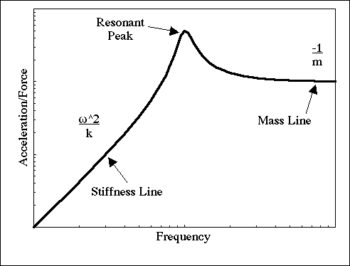
The FR of a structure reveals the natural frequencies of the structure; the natural frequencies correspond to resonant peaks in the frequency domain. As previously explained, very little force is required to excite the structure at a resonant frequency because the inertia and stiffness forces cancel. Consequently, the FR is at a maximum, and the damping of the structure is the only limiting factor to the magnitude of the response [6]. The characteristic form of the acceleration/force FR for a single resonant peak is shown in Figure 1.

Figure 1. Characteristic Form of Acceleration/Force Frequency Response at Resonance

The resonance in Fig. 1 occurs at the maximum in the plot. Prior to the peak, a mode’s response is primarily governed by the stiffness of the structure. The associated stiffness line, , increases at a slope of 2 on a log plot. Conversely, after resonance the affective inertance, or , of a mode provides the dominate response characteristic. The FR of the mode asymptotically decays to the modal inertance, often called the mass line. Both the stiffness and mass lines affect the overall FR when multiple resonances exist in a system. When a structure contains more than one resonant peak, the FR is a summation of all the resonances and their associated stiffness and mass lines.

The effect of the individual mass and stiffness lines is a factor that must be considered in modal analysis. When a restricted frequency range is viewed, one which does not include all of the resonant peaks of a system, the mass lines and stiffness lines from the resonant peaks outside of the frequency range still contribute to the overall FR of the system. These effects must be accounted for in order to produce an accurate mathematical model of the structural behavior. The theory of residuals accounts for this phenomenon and is presented in section 2.7.4.

The method of supporting a structure during vibration testing has a direct impact on the modal characteristics of the structure. The two types of idealized supports for vibration testing include a constrained support and a free support. In actuality, neither of these idealized supports are physically realizable. Free support consists of the structure floating free in space with no support attachments, whereas constrained support requires a fixed attachment to some other structure that exhibits no base motion [7]. The selection of the constraint is subject to the operating environment of the structure. Since the normal operating environment for an aircraft is flight, the free-support system is chosen for most GVT’s.

The free system is approximated by placing the system on a very soft cushion. The cushions approximate the free constraint by damping out high frequency vibration from external sources such as the building, test environment, or other external sources. However, the tires will vibrate at low frequencies due to a small amount of friction between the tires and test structure. From structural dynamics theory, rigid-body modes of a free structure occur at zero frequency [6]. The friction in the free supports affects the FR of the structure and causes rigid modes to exist at very low frequencies other than zero. If the cushion is soft enough, rigid body modes are well below the first flexible modes of the structure and are negligible to the overall FR. According to the FAA, an aircraft in a GVT should be supported such that rigid-body modes occur at frequencies less than 1/4 of the first flexible mode [9]. Other sources claim that the highest rigid-body mode should be at a frequency less than 1/10 of the first flexible mode [7].

Since the aircraft is a three-dimensional structure and has no constraints governing the directions of deformation, the structure has six degrees of freedom. These six degrees of freedom make up the six rigid-body modes inherent to the aircraft: roll, pitch, yaw, longitudinal translation, lateral translation, and vertical translation (Fig. 2).

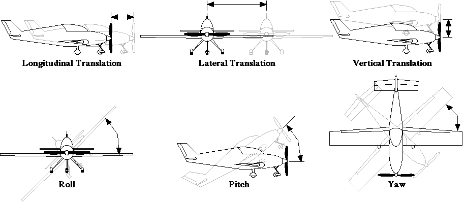
Figure 2. Visual Representation of the Six Rigid-Body Modes of the Star-Lite Aircraft

The presence of the rigid-body modes in the free support has an impact on the FR of the structure. These effects must be accounted for in the mathematical models of the structural response and are often dealt with by the theory for residuals; again, an explanation of residuals will be provided in section 2.7.4.

The methods of exciting a structure and taking measurements for modal analysis are subject to many variables. These variables break down into the basic categories of excitation of a structure, determination of an excitation frequency range, and determination of a node layout for GVT measurements. Although the topics can be separated into categories, each is interrelated.

The variables involved in the excitation of a structure include the type of excitation signal to be used, the means of producing a physical input excitation, and the method of transferring the physical excitation to the structure.

The determination of the excitation signal to be used in a GVT is based on the theory behind FR’s. If a structure is linear, the FR is independent of the type of stimulus used to excite the structure [10]. Based on this statement, any form of input excitation could be used for the modal analysis of a structure. However, most structures exhibit some form of nonlinear behavior at certain excitation frequencies or amplitudes. If nonlinearities are of concern in a GVT, a burst random signal is the best choice for the excitation signal. Burst random excitation does not characterize nonlinearity well and can be used to estimate the best linearized model of a nonlinear system [7]. In addition, random excitation of the structure will produce modal frequency responses of the modes at all points on the structure because random noise spans all frequencies .

Burst random signals provide the benefits of both impulse and continuous random testing [11]. Burst random signals are self-windowing; like an impulse, the burst random input is a transient response that decays within the time window. Burst random signals also provide an observable input response; like a continuous random signal, burst random signals provide multi-frequency inputs and a good linearized model. Finally, burst random inputs require less FR averages [11].

A single input excitation is usually adequate to excite all the modes of a small structure. However, when using a single excitation source, nonlinearities in structural response can result from an excessive excitation amplitude. Thus, the amplitude must be kept small and the data must be monitored to ensure few nonlinear elements are being excited. If the amplitude required to avoid nonlinear responses is too low to excite a structure, a multi-input excitation must be considered [11].

The length of an excitation burst is also a major contributor to the quality of FR data. In order to accurately compute the FR of a structure, the response of the signal must decay within the sampling period of the test; the signal decay and sampling period are discussed in section 2.6.1 on the discrete sampling of complex signals. As the length of the random excitation burst increases, the amount of excitation of each frequency also increases. The FR improves because more data is available at each natural frequency. The method for determining a proper excitation burst length involves exciting the structure for different lengths of time and observing the response of the signals. If the signals decay prior to the end of the sample period, then the excitation burst length is appropriate for testing. In order to ensure that the signal will decay within the sample period for every measurement, the burst length should be conservatively selected in order to account for measurement positions at which the response may decay more slowly.

The most common piece of hardware to produce an excitation is an electro-magnetic shaker. The shaker takes the input voltage from a burst random signal and transforms the voltage to a physical motion of a flexible plate. In order to avoid forces being transferred between the base of the shaker and the structure, the shaker must be isolated from the structure [7]. Isolation of the shaker is not always possible; however, the use of some sort of dissipative material to support the shaker can aid in reducing the transmission of forces through the base. For example, a thick foam support can help to damp out shaker excitation of a common shaker-structure base such as the floor.

Most shakers operate over a frequency range of 5 Hz - 20 kHz. For a softly supported structure, the rigid-body modes are often in the range of 0 Hz - 3 Hz; hence, a FR will not provide information on the rigid-body modes. Instead, in order to determine if the rigid-body modes are well below the first flexible modes, the frequencies of rigid-body motion must be determined in some other manner. The rigid-body modes of a softly supported structure can be determined by physically pushing on the structure at a resonance frequency; the resonant frequencies are generally low due to the soft supports and are easy to excite by hand.

In order to transfer all of the excitation force through an axial load cell, the forces need to be applied in a single axial direction. The use of a flexure rod and stinger provides a means of transmitting an axial load without forces or moments in other directions. The stinger is a thin, slender rod that is axially rigid but bends easily. The natural bending of the stinger helps to decrease the transmission of non-axial loads. The flexure is also a rod or hollow tube, but is much thicker than the stinger and has a higher stiffness. The flexure is used to transmit the loads between the stinger and structure without causing the setup to buckle under load. In order to minimize the presence of external forces or bending entering the structure, a stinger is often placed on both ends of the flexure. This assembly is commonly referred to as a flexure fixture (Fig. 3).

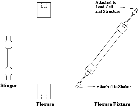
Figure 3. Typical Configuration of a Flexure Fixture

The transfer of input excitation from the shaker to the structure is accomplished through attachment of the flexure ends to both the shaker and the structure. The input force is measured by a load cell that is attached between the flexure and structural mounting point.

The method of attachment to the structure depends on whether or not the test is being conducted in a non-destructive manner. For non-destructive tests, a common method of attachment involves the use of a suction plate attached to the end of the flexure fixture. The suction plate is attached to a pump that provides a vacuum to keep the plate attached to the surface of the structure. The point of attachment on the structure depends on an analysis of the structural nodes, which will be discussed in the next section.

Since the natural frequencies of a structure are independent of the location on a structure, determination of a range for modal testing is a fairly straightforward task. Given a specified shaker location, the excitation range for the GVT is found by measuring the FR at several points on the structure and comparing the frequencies that exhibit structural resonance. The selection of the highest significant resonance is based primarily on good engineering judgment. Before a selection is made, the FR should be taken at several combinations of different shaker and accelerometer locations to ensure the measurements were not taken at points corresponding to structural nodes.

Although the natural frequencies of a structure are excited at every measurement point, their associated mode-shape amplitudes differ depending on the point of the measurement. The different amplitudes are caused by the shape of the mode at the measurement point [10]. Fig. 4 displays an example of the first two mode shapes found in a rigidly-supported cantilever beam.

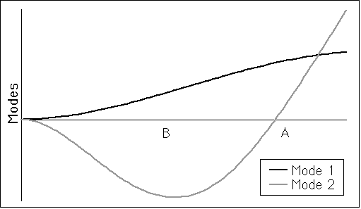
Figure 4. First Two Mode Shapes of a Cantilever Beam

The mode shapes in Fig. 4 illustrate the different mode deflections along the length of the beam. A point associated with no modal deflection is known as a node point. Point A in Fig. 4 displays an example of a structural node for the cantilever beam. If a shaker is placed at a structural node, the mode shape corresponding to the node will have an excitation input of zero. Similarly, an accelerometer placed on a structural node will not receive any vibration from the associated mode. Point B in Fig. 4 corresponds to a position at which both modes have significant amplitudes. The best method for finding the modal frequencies in a structure is to take measurements at several locations for both the shaker and accelerometer in order to identify each modal frequency. Once all of the modal frequencies are identified, the shaker is set at a location that produces excitation of all the modal frequencies.

In order to obtain the mode shapes and modal parameters of a structure, measurements of the response of the structure to a known input must be recorded at many discrete points on the surface of the structure. The combination of all discrete points on the structure is commonly referred to as the node layout. The determination of the node layout is a delicate and tedious task, but proper selection allows for assembly of FR data from each discrete point that provides enough information to adequately determine mode shapes and modal parameters. Improper selection of the discrete points in the node layout can cause inaccurate characterization of mode shapes and improper calculations of the significant modal parameters. The selection is primarily based on experience and good engineering judgment, but the underlying requirement is to choose enough points in order to accurately reproduce the shape of the mode.

The selection of points for modal testing is analogous to the Nyquist Criterion in digital signal analysis (A discussion of the Nyquist Criterion is found in Appendix A). If too few points are chosen, the points do not adequately collect information on the shape of the structure during modal deformation. Conversely, if enough points are chosen, the resulting responses of the structure will accurately measure the shape of each mode. Figure 5 shows an example of improper node layout selection versus a more accurate representation. The discrete points are connected to illustrate the spatial aliasing that can occur from improper node-layout selection.

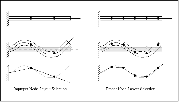
Figure 5. Examples of Node Layout Selection

The beam on the left side of Fig. 5 shows an example of an improper node layout. The two node points do not accurately represent the shape of the beam. However, the beam in the right-hand portion of Fig. 5 has a proper node layout, and the node points provide enough information to reproduce the deformed shape of the beam. The measurement accuracy of mode shapes increases with the number of discrete points chosen for measurement. The natural inclination would be to select as many points as possible in order to ensure complete coverage of all mode shapes; however, if too many points are selected, the resulting measurement and computation time is extremely long.

A convenient method for determining adequate node point spacing is suggested in [10]. The first step is to take the FR of a few points to determine the highest significant frequencies present in the structure, as mentioned in section 2.4.2. After the highest significant modal frequency is determined, the stimulus is moved away from the initial position through small increments. The FR measurement is repeated and the amplitudes of the highest frequency are tabulated and plot versus the displacement from the initial position. For higher modes, the plot of the data should display a harmonic-type response similar to that in Fig. 5. One cycle of the harmonic response represents the 360° phase shift described in [10]. The 360° shift is similar to a single period in a sine wave.

Figure 4 shows only one structural node in Mode 2 and no type of sinusoidal pattern because mode shapes are generally not symmetric about their undeformed axis [6]. This phenomena indicates that a 360° shift would not occur when measuring the second mode’s phase shift along the beam. However, at higher modes, the number of structural nodes is one less than the chronological rank of the natural frequency: the rank is based on the chronological order of resonant frequencies starting with the first flexible mode [6]. Therefore, since most structures have several significant modes, and consequently several structural nodes, the sinusoidal approximation for the 360° shift offers a systematic method for determining the measurement point spacing. In order to ensure that the 360° phase-shift method properly discretizes the mode shape, the distance measured between the start and end point of the shift should be separated into five or more increments. Additionally, several measurements should be taken across several structural components in order to determine the resolution needed to find the mode shape across the entire structure. The interactions at spar and rib junctions are also of special interest because of their effect on the FR and mode shapes of the structure [10].

The natural frequencies of a linear structure are independent of the location on a structure, as discussed in section 2.4.2. Based on the linearity assumption, a single excitation point is sufficient to excite the structure such that response measurements at all other points provide enough information to compute the natural frequencies, damping, and mode shapes of the entire structure [7]. In addition, Maxwell’s Reciprocity Theorem for a linear system states that an excitation at point x and a response at point y is equal to the same excitation at point y and the response at point x [7]. Maxwell’s Reciprocity Theorem provides a means of validating the linearity assumption in the GVT of a structure. Figure 6 presents the typical method for testing a structure according to Maxwell’s Reciprocity Theorem.

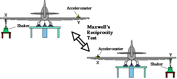
Figure 6. Applying Maxwell’s Reciprocity Theorem to Testing

The resultant FR data from a Maxwell’s Reciprocity test (Fig. 6) can be compared over the frequency range of interest in order to determine the validity of the linearity assumption for a structure undergoing vibration testing.

A quality modal analysis of a structure must account for the many sources of potential error in FR measurements. Most modal analyses use a DSA (Dynamics Signal Analyzer) to perform calculations of FR’s from the response data of the structure under test. Many of the sources of error in data come from the improper discrete sampling of data; therefore, the potential errors should be presented with the theory behind data analysis. This section begins with the benefits associated with the use of a DSA for discrete sampling. The concepts of coherence, averaging, and amplitude ranging are then presented in order to show how a DSA can be used to deal with many of the problems in data analysis.

The use of the frequency domain for testing provides a convenient method for determining the mode shapes, as well as the resonant frequencies of a structure. The resulting modal parameters provide a method for determining the structure’s dynamic response to any arbitrary excitation [12]. Unfortunately, the FR method is extremely sensitive to the properties of discrete sampling, and improper selection of sample rates can lead to problems such as aliasing and leakage in the FFT (Fast Fourier Transform) of the actual signal.

The most common method in modal analysis for analyzing complex signals is through the use of a DSA (Dynamic Signal Analyzer). The DSA creates the source signal for a modal test and also acquires the output data. Additionally, the DSA performs the first step of the data analysis. The DSA produces the complex signals that are input to a shaker. The shaker then produces an output force that is transmitted to the structure through the flexure fixture, and the input force at the shaker location and corresponding output accelerations of discrete points on the structure are measured by a load cell and accelerometer. The outputs from these instruments are fed back into the DSA which then digitizes the complex signals by sampling them at discrete points in time. The data is transformed into the frequency domain through a FFT.

The number of samples and duration of sampling is set through the DSA. The number of samples is usually based on a power of 2 in order to optimize the FFT of the signal [10]. Analysis of the resulting discrete data is known as digital signal processing. Although much of the fundamental criteria for proper discrete sampling is handled intrinsically by the DSA, an understanding of the fundamental concepts is necessary when performing a GVT. These fundamental concepts include: periodic signals, FFT (Fast Fourier Transform), time domain, frequency domain, sampling frequency, block size, leakage, and aliasing. The basic concepts are presented below, but a mathematical analysis of these properties is presented in detail in Appendix A.

Frequency response data is calculated with a FFT, which assumes the sampled signal is periodic in the time sample of interest. For periodic signals, a FFT produces a frequency spectrum with vertical spikes at the frequencies present in the signal; however, when non-periodic signals are input to a FFT, the resulting frequency spectrum contains leakage into frequencies that are not present in the original signal. For the GVT, the burst random input produces a transient response single. A transient signal is valid in a FFT because the signal decays prior to the end of the time period. The FFT is essentially tricked into thinking the transient signal is periodic; hence, no information is lost in conversion to the frequency domain and leakage is absent. The leakage-free phenomena is a benefit of the burst random signal.

Discrete sampling of complex signals requires proper knowledge of the frequency content of a complex signal. Improper discrete sampling of a complex signal can lead to a phenomena known as aliasing, which transforms the actual frequency of a signal to a lower frequency. This phenomena is similar to the misrepresentation of the mode shapes shown in Fig. 5. Proper discrete sampling requires careful selection of the sampling frequency in order to obtain enough data to capture the highest frequency present in the wave. The concept of the Nyquist criterion, which governs the selection of the sampling frequency, states that a signal must be sampled at a rate of more than twice the highest frequency in order to obtain accurate information. In addition, the block size or number of frequency lines of the sample provides the fundamental frequency of the discrete signal and must be properly selected in order to obtain the lowest frequency in the complex signal. The DSA uses the frequency span of interest to automatically set the sampling rate at more than twice the highest frequency chosen, and the chosen frequency resolution then accounts for the block size of the samples. Further information about a DSA can be found in [13].

The coherence function provides a method for determining the quality of FR data, and is based on information obtained from the FFT of a time-domain signal. Coherence relates the system output power directly related to the input [14]. Coherence is based on a scale of 0 to 1 where a 1 represents perfect coherence: all of the output was produced by the input. Conversely, a coherence of 0 indicates there is no relationship between the input and output power. At coherence values between 0 and 1, the output is receiving information from sources other than the input. These other sources can include noise contamination from the environment, base motion of supports, nonlinearity of the structure, bad connections, and even resonance frequencies of a structure.

In order to obtain good coherence in a test, the DSA should be configured to average data over several FR’s. If only one FFT is calculated, the coherence function provides a value of 1 because the function assumes all of the output power is produced by the input [14]. A common form of averaging is a simple linear averaging of each FR measurement. In order to obtain a 90% confidence that the FR data is within certain limits, the data must be averaged a minimum of 16 times [14]. After all 16 averages, coherence measurements above 0.9 will indicate that FR data is within +1.1 dB and -1.3 dB of the actual value. Coherence measurements less than 0.9 have a less accurate range. Averaging more than 16 signals further increases the confidence range, and [14] provides a table of the accuracy based on the number of averages and the measured value of coherence. For a derivation of the Coherence function, refer to the information presented in Appendix B.

At a resonant frequency of a structure, the amplitude of the FR depends only on the damping in the structure, as mentioned in previous Theory sections. At a resonance, very little force is required to produce a response. The result is a drop in the input-force amplitude at the resonance, which can result in the measurements being more susceptible to noise [7]. Any increased noise has the affect of decreasing the coherence around resonant peaks. Additionally, structures with loose parts will exhibit a drop in coherence due to the nonlinear vibration of those parts. In theory, the mean value of random noise tends toward zero as the number of averages of a signal increases. For systems with nonlinearities, averaging time records is helpful in decreasing the noise and increasing statistical reliability [7]. Additional increases in coherence can be obtained through the constraint of loose components in order to reduce nonlinear vibration.

Even though the primary cause of coherence loss in a test is due to noise and nonlinear effects in a structure, another source of error can come from the range setting on a DSA. The phenomena of over-ranging and under-ranging cause additional noise in FR measurements and a drop in the coherence of the data. Over-ranging a signal involves setting the DSA range for a transducer at levels much higher than the actual signal. Over-ranging results in a noisy FR measurement and poor coherence [7]. Under-ranging a signal involves setting the amplitude range below the actual magnitude of the signal response. This causes overloading of the DSA and again poor FR data and coherence result.

Most DSA’s are set to reject overloads in order to minimize the loss of data due to under-ranging; however, in order to avoid over-ranging, the range of the DSA must be set through examination of the actual signal responses. The optimal range setting is twice the maximum amplitude of the signal. This type of configuration is known as half-ranging and makes efficient use of the dynamic range of the analog-to-digital converter in the DSA [7]. When half-ranging is incorporated into testing, the coherence and FR are much smoother than cases that have over-ranging and under-ranging of signals.

The Test application of I-DEAS software provides an interactive tool in modal analysis. The application integrates FR data from actual tests into an analytic model of the test structure. The model of the structure must be constructed according to the coordinates of measurement points used during testing in order to match each FR with a corresponding measurement point. Once the FR data is integrated into the analytic model, the Test application is used to estimate the model parameters from a curve fit of the FR data. The remainder of this section describes the polyreference curve-fitting technique and some computational parameters used in the analysis of the Star-Lite GVT data. In addition, a comparison of modal damping versus structural damping and the theory of residuals are introduced in order to eventually clarify the analytical results.

The polyreference technique is a two-stage modal estimation method developed by H. Vold at SDRC. The polyreference technique is valid for data containing single or multiple excitation references. The technique is formulated for free-decay and impulse-response data. The first stage of the polyreference technique uses a curve fit to approximate the time-domain signal of a response in order to extract the natural frequency and modal damping of each mode. The second stage uses either a time-domain or frequency-domain technique, specified by the user, to calculate the residues and modal coefficients of each mode shape in the structure [5].

The polyreference technique produces data for measuring the validity of modal parameters calculated from FR data. The first stage of the polyreference technique generates a MCF (Modal Confidence Factor) for each estimate of natural frequency and modal damping. The MCF provides a measure of the physical significance of each mode. During the estimation of the modal parameters, the polyreference technique generates computational and physical modes. The MCF provides a value of 1 for physical modes and a value of 0 for computational modes. Values between 0 and 1 indicate less certainty of the physical significance of a mode. Consequently, the final selection of the mode is subject to good engineering judgment [15].

The MAC (Modal Assurance Criterion) is a matrix of values between 0 and 1 that are used to determine the linear independence of mode shapes calculated in the second stage of the polyreference technique. A value approaching 0 in the MAC indicates that two mode shapes are linearly independent. Conversely, a value close to 1 indicates that two modes are linearly dependent. The diagonal of the MAC matrix is 1.0 since all modes are linearly dependent on themselves. The off-diagonal values of the MAC indicate the dependence of each mode on every other mode. If the off-diagonal values are 0, the modes are linearly independent; however, as the MAC value increases above 0, the degree of linear dependence between two modes also increases. MAC values above 0 can indicate

Although the MAC provides a measure of the linear dependence of modes, the MAC is not a true orthogonality check because the structural mass and stiffness matrices are not considered in the MAC formulation. However, the MAC provides a first-run attempt at determining the linear independence of mode shapes [15].

The first stage of the polyreference technique produces estimations of both the natural frequencies and modal damping factors for each mode in a structure. The modal damping parameter is often confused with the structural damping factor, which is typically used in other aeroelastic analyses such as flutter analysis. This section will provide a brief derivation to relate the structural damping factor to the modal damping factor. The information in this section was provided by Dr. Ron O. Stearman [9].

The characteristic differential equation describing a mass-spring-damper system is given by

(Eq. 2.7.3.1)

where

The values of the natural frequency (w _n) and modal damping (g ) are expressed through the following relationships:

(Eq. 2.7.3.2)

(Eq. 2.7.3.3)

Equation 2.7.3.1 is solved by assuming a harmonic solution of the form

(Eq. 2.7.3.4)

where

Substitution and manipulation of Eqs. 2.7.3.2, 2.7.3.3, and 2.7.3.4 in Eq. 2.7.3.1 produces a convenient form for comparing modal damping to structural damping:

(Eq. 2.7.3.5)

The standard form for the structural damping factor used in flutter analysis is given by

(Eq. 2.7.3.6)

where

g = structural damping factor.

A comparison of Eqs. 2.7.3.5 and 2.7.3.6 indicates

(Eq. 2.7.3.7)

when the harmonic frequency (w ) is equal to natural frequency (w _n).

Actual analysis of physical systems does not allow the characterization of all the mode shapes and modal parameters due to the infinite number of natural frequencies and modes. Residuals account for the dynamics outside the test frequency range that affect the data within the FR of that range [16]. Basically, the theory of residuals examines the mass lines and stiffness lines from frequencies outside of the obtainable frequency range or the frequency range of interest.

Before the theory of residuals can be applied, a mathematical model of the FR must be obtained from actual test data taken at the discrete measurement points on a structure. The mathematical model uses the information from each FR to reconstruct a representation of the individual contributions from each resonant frequency. The mathematical model only represents the FR’s of modal frequencies present in the frequency range and does not contain the information from the mass lines and stiffness lines entering the frequency range from other modes. The basic process followed by residual theory involves subtraction of the mathematical model of the FR from the original FR data taken at each discrete point on the structure. The resulting data consists of the combined mass lines and stiffness lines of frequencies lower and higher than the frequency range of the data, respectively [16].

The most common method for determining the inertance and flexibility residuals outside of the test frequency range is the subtraction of the mathematical FR model from the actual test model. When the physical structure is available for further testing, [16] suggests other methods for determining the inertance and flexibility residuals. The most convenient alternate method is one for the flexibility residual that involves a second FR taken at each discrete point. The second FR is taken over a slightly higher frequency range than the original test frequency range in order to obtain a few higher modal frequencies. These extra modes are considered the primary contributors to the flexibility residual in the original test frequency range and can be used to account for the out-of-band modes [16]. The other methods for inertial and flexibility methods are not as convenient and the reader is referred to [16] for more detail.

An additional note needs to be made in regards to the mass lines associated with a GVT on a freely-supported structure. For a freely-supported structure, the rigid-body modes occur at frequencies other than zero. The mass line (also known as the inertia restraint) in the FR has additional contributions from the low frequency responses of the rigid-body. The information in [16] provides some potential methods for independently determining the effect of the rigid-body modes, but the reader is again referred to the document for information on this method.

The use of accelerometers and load cells allows engineers to determine the relationship between the input forces and output accelerations present in dynamic systems. In order to obtain useful data from an accelerometer/load-cell pair, the measurement devices must be calibrated. The use of ratio calibration allows the simultaneous calibration of both sensors. Individual calibration of each sensor can introduce cumulative errors associated with the separate calibration standards used for each instrument [17]. Ratio calibration bypasses the use of calibration standards by simply providing the ratio of the accelerometer output to the load-cell input.

Ratio calibration requires the use of a hanging weight of known mass with the accelerometer attached on one end. For the common impact-hammer test, the load cell is attached to an impulse-force hammer, which is used to impart an impulsive force on the mass. An example of the setup for a ratio-calibration is given is Fig. 7.

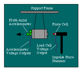
Figure 7. Configuration for a Ratio-Calibration Experiment

Both the impulse force and the accelerometer output are measured in order to develop a calibration ratio based on acceleration, force, and the mass of the hanging-weight/accelerometer combination. The calibration ratio is also based on the FR of the accelerometer/load-cell voltage responses. The calibration ratio between known mass and the accelerometer/load-cell voltage ratio is

(Eq. 2.8.1)

where

R = calibration ratio

= ratio of accelerometer/load-cell amplifier gains

= ratio of accelerometer/load-cell output voltages

m = mass of hanging weight.

Once the calibration ratio is determined, the voltage ratios from a test that uses the same accelerometer/load-cell pair can be used to determine the inertance (acceleration/force) for the actual test. From ratio calibration theory, the inertance is given by

(Eq. 2.8.2)

where represents the ratio of the accelerometer/load-cell voltage from the actual test.

A thorough mathematical development of the ratio-calibration formulas is provided in Appendix C.